In this post we will implement Churn Model Prediction System using the Bank Customer data.

Using the Bank Customer Data, we can develop a ML Prediction System which can predict if a customer will leave the Bank or not, In Finance this is known as Churning. Such ML Systems can help Bank to take precautionary steps to ensure the customer stays with the Bank.

Importing the Necessary Libraries

Lets start by importing the necessary libraries needed to execute this project.

import tensorflow as tf
from tensorflow import keras
from keras.layers import Dense
import numpy as np
import pandas as pd
import matplotlib.pyplot as plt

%matplotlib inline

The problem that we are trying to classify is a binary classification problem.
In every ML Problem we need to clean the data, preprocess the data and split the data for train and validation, so lets import necessary libraries for those tasks.

from sklearn.preprocessing import StandardScaler, LabelEncoder
from sklearn.utils import shuffle
from sklearn.model_selection import train_test_split

Loading the Data

We will use google colab for this project, let’s load the dataset from kaggle on to colab, follow the link if you dont know how to load kaggle data onto colab.

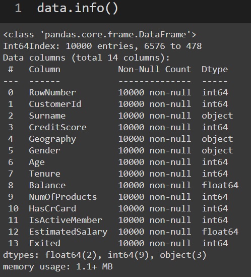
Once the data is loaded we can use the panda’s head function to look at the data and info function of panda’s to have a glance at the column types and if there are any null values present. Luckily this dataset is clean and there are no null values present.

Preprocessing of data

It is very important to shuffle the data before we begin with preprocessing of the data.
The shuffle function of scikit-learn will shuffle the data for us.

data = shuffle(data)

Preprocessing involves steps like

• Checking for null values
• What columns to be used and what to be dropped
• Converting categorical values to numerical values
• Normalization or Standardisation of the column data

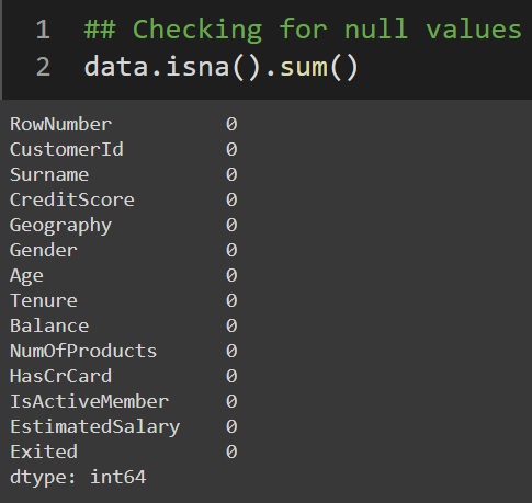
Check for NULL Values

using the below pandas functions we can get the number of null values present in each column of the dataset.

data.isna().sum()

As you can see from the below graph, All the columns report zero, indication there are no null values in the dataset.

Selecting important columns

Pandas columns attribute will list the column names, the CustomerId, Surname and RowNumber are not very helpful for our model. The Exited column is a target column

data.columns
X = data.drop(['RowNumber','CustomerId','Surname','Exited'], axis=1)
y = data['Exited']

We will split the dataset into X and y, where X is input and y is target variable.

Categorical to Numerical

The pandas dtype returns a series with the data type of each column. We can see that the ‘Geography’ and ‘Gender’ are categorical columns.

X.dtypes
X['Geography'].unique()
X['Gender'].unique()
X = pd.get_dummies(X, prefix='Geography', drop_first=True, columns=['Geography'])
X = pd.get_dummies(X, prefix='sex', drop_first=True, columns=['Gender'])

The pandas unique function return a series listing the unique values of each column. We will use pandas get_dummies function to convert the categorical columns into numerical columns.

Applying standardisation

We will apply standardisation, so no column has more effect on the output than other columns. It scales all values between -1 and 1

scalar = StandardScaler()
X = scalar.fit_transform(X)

Creation of Training and Validation datasets

Using the train_test_split we will create training and validation datasets, until the model is final we should not use the test datasets.

X_train, X_test, y_train, y_test = train_test_split(X,y,test_size=0.3, random_state=42)

NN Model Building

Now that the data is ready, we can build a NN (Neural Network) model, we can start simple and use a 1 or 2 hidden layers. In this for demostration purpose we will build a 4 hidden layers model. You can change the model and fine tune it to learn better using more layers and experimenting with different nodes in each layer.

model = tf.keras.models.Sequential([
Dense(256, activation='relu', input_shape=x_train.shape),
Dense(128, activation='relu'),
Dense(64, activation='relu'),
Dense(32, activation='relu'),
Dense(1, activation='sigmoid'),
])

We are using Sequential model here and the dense layers, the activation function used is relu, since this is binary classification problem we have used sigmoid as the activation function in the last layer.
We can use the summary function to have a look at our model and its network

model.summary()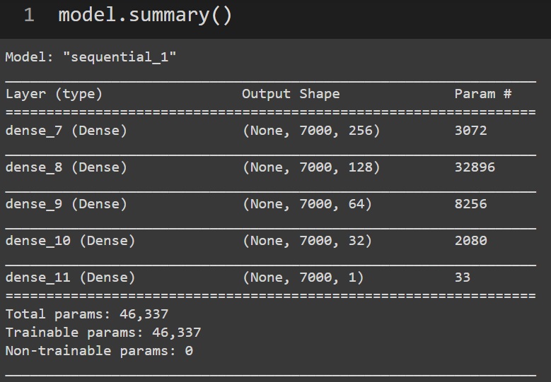

Compile and fit the model

model.compile(loss='binary_crossentropy', optimizer='adam', metrics=['accuracy']
history = model.fit(X_train, y_train, verbose=1, epochs=50, batch_size=32, validation_data=(x_test, y_test))
)

Plotting the model accuracy and loss plots

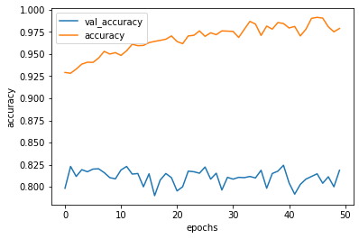
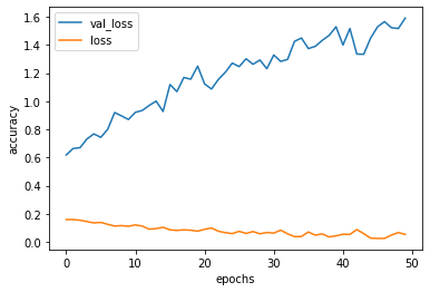
From the graphs we can see that the validation accuracy is around >80% not bad for a simple model.

Conclusion

In this problem we have used a simple 4 layer model to come up with a prediction system, the model is certainly overfitting ( the validation loss keeps increasing). There is lot of scope to improve this model further.

Further Improvements

• We can add dropout layers to make model less overfit
• Use callbacks to stop model learning once the accuracy stops getting better
• Experimenting with different nodes and hidden layers.

Different Dataset same problem

Use the telco dataset and see if you can use the same model to predict if a customer will leave their telecom network or not.

Source Code

Checkout the full Source Code of the above project.

References

• Artificial Neural Network using Tensorflow 2 Book.
• TensorFlow website